Info
- 任务目标
- 搭建 GPT 2 模型(最小参数)
- 可以调用训练好的 GPT 2 参数
- 实现 next word 预测
- 能够从零开始训练模型
搭建模型
GPT2 的模型可以被简化为如下模块构成:
class GPT(nn.Module):

    def __init__(self, config):
        super().__init__()
        self.config = config

        self.transformer = nn.ModuleDict(dict(
            wte=nn.Embedding(config.vocab_size, config.n_embd),
            wpe=nn.Embedding(config.block_size, config.n_embd),
            h=nn.ModuleList([Block(config) for _ in range(config.n_layers)]),
            ln_f=nn.LayerNorm(config.n_embd)
        ))

        self.lm_head = nn.Linear(config.n_embd, config.vocab_size, bias=False
它们的关系可以用下图表示:
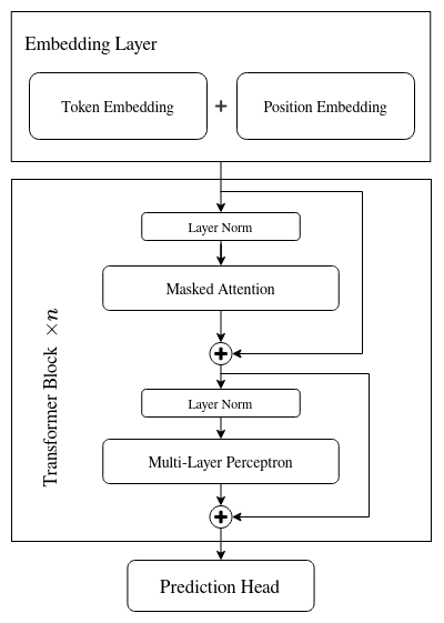
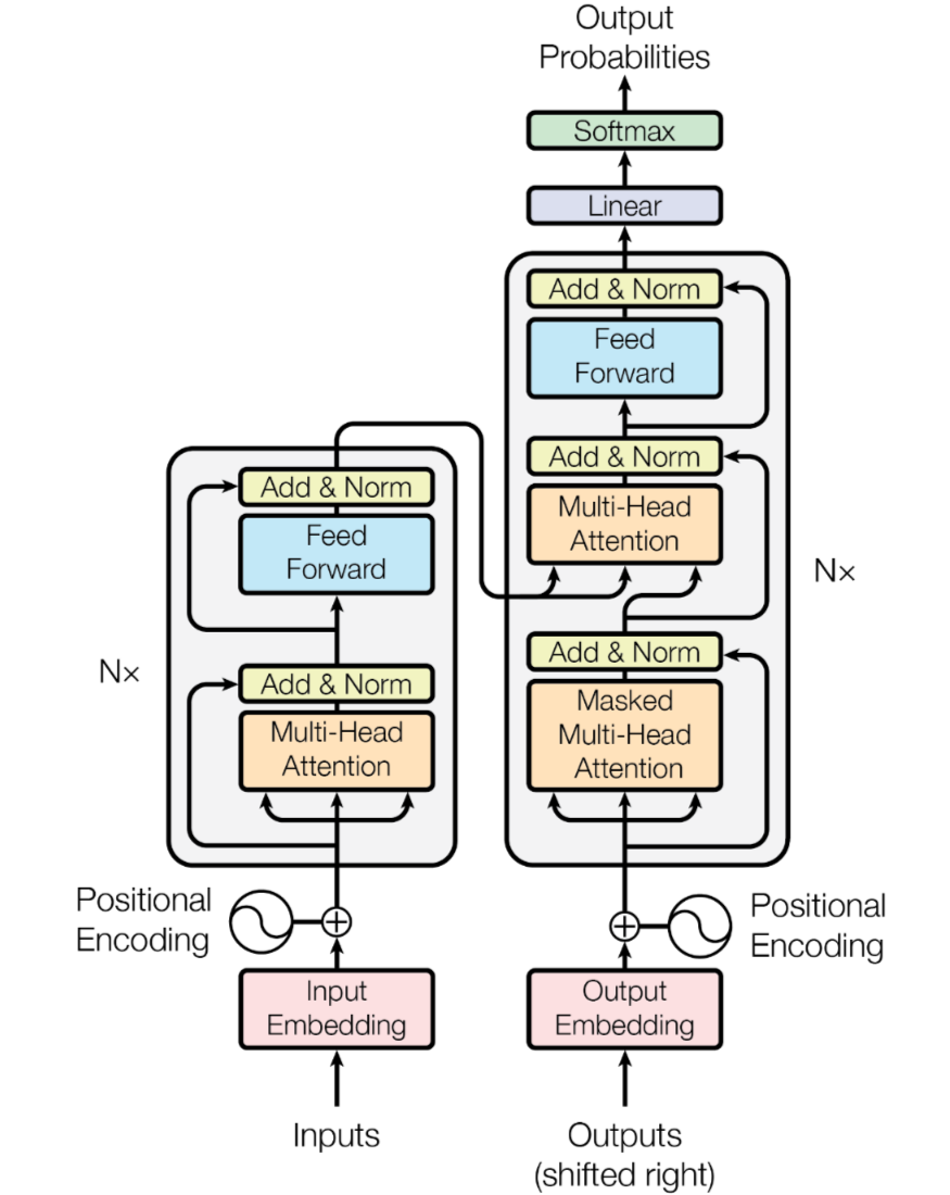
Embedding 层使用了两个 Embedding Layer,目标是让模型从数据中学习到 token 和位置的正确表示。Transformer Block 使用了源论文的 Decoder 部分,需要注意的是,GPT2 使用的 Decoder 与 Attention is all you need 这篇文章中 Layer Norm 的位置有所不同(GPT2 中是 NormAdd,Transformer 中是 AddNorm),并且只保留了 Masked Attention 和最后的 Feed Forward,前者更注重对输入的标准化,而后者则是在生成过程中处理输出的稳定性。:
GPT2 的默认权重是 Tensorflow 格式的,为了在 Pytorch 中使用预训练的权重,需要对权重进行转换:
@classmethod
def from_pretrained(cls, model_type):
	assert model_type in {'gpt2', 'gpt2-medium', 'gpt2-large'}
	from transformers import GPT2LMHeadModel
	print(f'loading pretrained {model_type} model...')

	config_args = {
		'gpt2': dict(n_embd=768, n_layers=12, n_heads=12),
		'gpt2-medium': dict(n_embd=1024, n_layers=24, n_heads=16),
		'gpt2-large': dict(n_embd=1280, n_layers=36, n_heads=20),
		'gpt2-xl': dict(n_embd=1600, n_layers=48, n_heads=25),
	}[model_type]

	config_args['vocab_size'] = 50257
	config_args['block_size'] = 1024

	config = GPTConfig(**config_args)
	model = GPT(config)
	sd = model.state_dict()
	sd_keys = sd.keys()
	sd_keys = [k for k in sd_keys if not k.endswith('.attn.bias')]

	model_hf = GPT2LMHeadModel.from_pretrained(model_type)
	sd_hf = model_hf.state_dict()

	# align keys
	sd_keys_hf = sd_hf.keys()
	sd_keys_hf = [k for k in sd_keys_hf if not k.endswith(
		'.attn.masked_bias')]
	sd_keys_hf = [k for k in sd_keys_hf if not k.endswith('.attn.bias')]
	transposed = ['attn.c_attn.weight', 'attn.c_proj.weight',
				  'mlp.c_fc.weight', 'mlp.c_proj.weight']

	assert len(sd_keys) == len(
		sd_keys_hf), f"mismatched keys: {len(sd_keys_hf)} != {len(sd_keys)}"

	for k in sd_keys_hf:
		if any(k.endswith(w) for w in transposed):
			assert sd_hf[k].shape[::-1] == sd[k].shape
			with torch.no_grad():
				sd[k].copy_(sd_hf[k].t())
		else:
			assert sd_hf[k].shape == sd[k].shape
			with torch.no_grad():
				sd[k].copy_(sd_hf[k])
	return model
@classmethod 这个注解有点像工厂方法,可以静态创建一个类,并且直接返回类自身
-
Q:为什么
lm_head中去除了 bias? -
A:这是一种常见的优化手段,减少了模型参数。因为在隐藏层中已经学习到了很多信息,使用 bias 差别不大
-
Q: 为什么
Transformer Block如此有效? -
A:Karpathy 对
Transformer Block的解释很有意思,他把一个Block看作一次“Reduce and Map”的过程,模块中QKV操作可以看作是在对信息进行Reduce操作,因为输入元素可以”看到”其他元素,并且以此更新自己的信息,相当于信息被压缩了;而在MLP阶段,输入元素通过一个全连接网络重整了自身,看不到其他元素的信息,因此是一个Map的过程。通过多次的信息“压缩-重整”,其实也类似人在处理数据的过程。 -
Q: 在 GPT2 中,是如何保证预测下一个词不会受到后面的词影响的(
Masked Attention是如何实现的)? -
A: 代码如下,主要是通过一个下三角矩阵来遮盖不需要的注意力,将无用的注意力设置为负无穷,即注意力分数为 0
class CausalSelfAttention(nn.Module):
    def __init__(self, config):
        super().__init__()
        assert config.n_embd % config.n_heads == 0
        # key, query, value projections for all heads, but in a batch
        self.c_attn = nn.Linear(config.n_embd, 3 * config.n_embd)
        # output projection
        self.c_proj = nn.Linear(config.n_embd, config.n_embd)
        # regularization
        self.n_head = config.n_heads
        self.n_embd = config.n_embd
        # not really a 'bias', more of a mask, but following the GPT naming
        self.register_buffer("bias", torch.tril(torch.ones(
            config.block_size, config.block_size)).view(1, 1, config.block_size, config.block_size))

    def forward(self, x):
        B, T, C = x.size()
        # nh = number of heads, hs = hidden size per head
        # calculate query, key, values for all heads in batch and move head forward to be the batch dim
        q, k, v = self.c_attn(x).split(self.n_embd, dim=2)
        k = k.view(B, T, self.n_head, C //
                   self.n_head).transpose(1, 2)  # (B, nh, T, hs)
        q = q.view(B, T, self.n_head, C //
                   self.n_head).transpose(1, 2)  # (B, nh, T, hs)
        v = v.view(B, T, self.n_head, C //
                   self.n_head).transpose(1, 2)  # (B, nh, T, hs)

        # causal self-attention; Self-attend: (B, nh, T, hs) x (B, nh, hs, T) -> (B, nh, T, T)
        att = (q @ k.transpose(-2, -1)) * (1.0 / math.sqrt(k.size(-1)))
        att = att.masked_fill(self.bias[:, :, :T, :T] == 0, float('-inf'))
        att = F.softmax(att, dim=-1)
        y = att @ v  # (B, nh, T, T) x (B, nh, T, hs) -> (B, nh, T, hs)
        # re-assemble all head outputs side by side
        y = y.transpose(1, 2).contiguous().view(B, T, C)

        # output projection
        y = self.c_proj(y)
return y- Q: LLM 如何实现输入相同,输出不同的?
- A:这个部分很有意思,我以前总是以为当
seed确定时,输出的结果也一定是固定的,但在 LLM 中输出并不是一句话,而是一个词,所以需要经过多轮输出构成一句话,在这个过程中,对每个词的预测取前 topk 个,在这 个中根据概率进行平均采样。因此哪怕是同一个输入,也会因为中间词的采样不同,回答的结果也会不同
# prefix tokens
enc = tiktoken.get_encoding('gpt2')
tokens = enc.encode("Hello, I'm a language model,")
tokens = torch.tensor(tokens, dtype=torch.long)
tokens = tokens.unsqueeze(0).repeat(num_return_sequences, 1)
x = tokens.to(device)

torch.manual_seed(42)
torch.cuda.manual_seed(42)

while x.size(1) < max_length:
    with torch.no_grad():
        logits = model(x)  # (B, T, vocab_size)
        logits = logits[:, -1, :]  # (B, vocab_size)
        probs = F.softmax(logits, dim=-1)  # (B, vocab_size)
        topk_probs, topk_indices = torch.topk(probs, 50, dim=-1)  # (B, k)

        ix = torch.multinomial(topk_probs, num_samples=1)  # (B, 1)
        xcol = torch.gather(topk_indices, dim=-1, index=ix)  # (B, 1)
        x = torch.cat((x, xcol), dim=-1)  # (B, T+1)
训练模型
Tip
在训练初始阶段,有一个 sanity check 可以检查参数的初始化效果: 如果是分类问题,在初始化时肯定希望每个类的预测概率都是相等的,因此,假设有 N 个类别,则
- Q:在训练过程中,为什么使
lm_head和token_embedding权重共享? - A:引入这种归纳偏差可以更快地收敛,有效减少模型参数量。这样做保证了输入和输出的 embedding 在空间表示上的一致性,同时节省了大量的参数。
模型参数的初始化很有意思,Linear 的 bias 会置为 0,weight 会被初始化为正态分布 std=0.02,合理的解释就是,GPT-2 训练了多个不同参数量的模型,如果使用数值稳定性,则需要满足 ,而 正好落在这几个参数量的中间值附近
def _init_weights(self, module):
        if isinstance(module, nn.Linear):
            # in gpt2, the bias of Linear module is initialized to 0
            torch.nn.init.normal_(module.weight, std=0.02)
            if module.bias is not None:
                torch.nn.init.zeros_(module.bias)
        elif isinstance(module, nn.Embedding):
            torch.nn.init.normal_(module.weight, std=0.02
加快训练速度
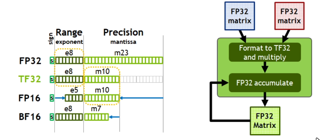
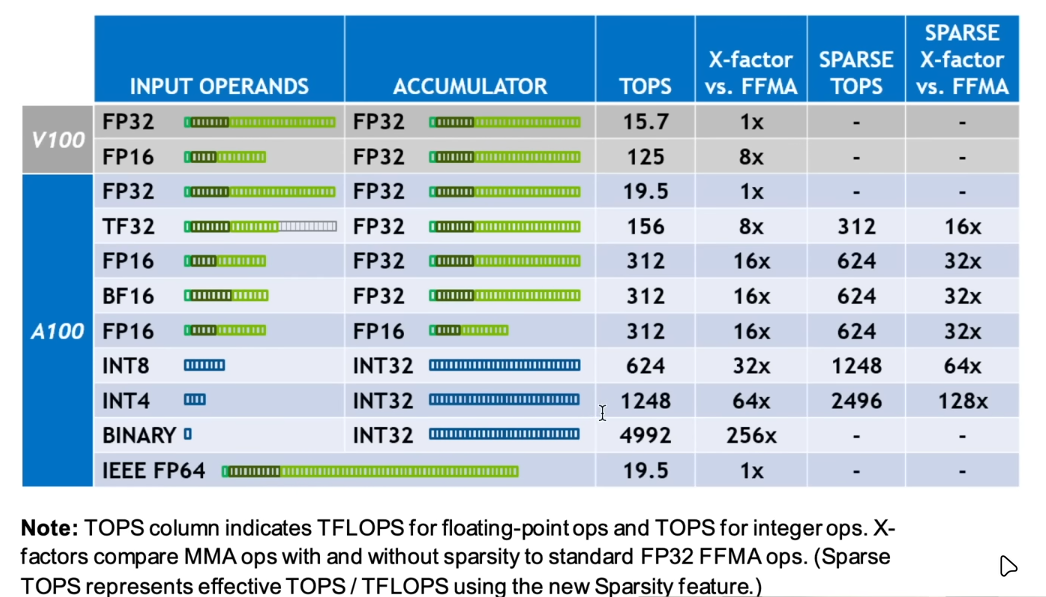
模型训练实际上需要消耗大量的存储空间,同时,为了 load 数据,中间的 I/O 需要消耗大量的时间,因此,想要加快训练速度,可以考虑调整数值精度。Pytorch 默认使用 FP32 来存储参数和计算,对于深度学习算法来说,数值精度对预测效果的影响不大,不如减少精度,可以明显提升训练速度。
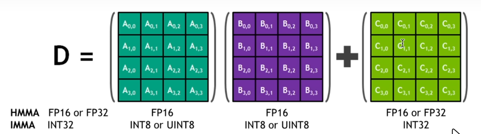
例如在半精度矩阵运算中,大块矩阵被分解为多个 的小块矩阵,通过多次执行乘法和累加操作,从而计算出大块矩阵的值(所以 batch_size 最好能被 4 整除)
- Q:如何评估训练速度?
- A:使用
time模块计算一个 batch 训练所需的时间。需要注意的是,在 GPU 上训练时,CPU 只负责分发任务给 GPU 队列,GPU 执行好后返回即可,但time()计算的是 CPU 顺序执行的时间,因此需要调用torch.cuda.synchronize()等待所有的操作完成再计算消耗时间
import time
for i in range(50):
    t0 = time.time()
    x, y = train_loader.next_batch()
    x, y = x.to(device), y.to(device)

    optim.zero_grad()
    logits, loss = model(x, y)
    loss.backward()
    optim.step()
    torch.cuda.synchronize() # only needed with CUDA
    t1 = time.time()
    dt = (t1 - t0) * 1000 # ms
    print(f'step {i}, loss: {loss.item()}, dt: {dt:.2f} ms')
在 GTX 3060 laptop 显卡中,每次读取的数据大小为:DataLoaderLite(B=8, T=128),取训练 50 步的结果 dt: 190.44 ms, tok/ms: 5376.94 为基准速度
step 1: Float32 Precision
在模型载入前运行:
torch.set_float32_matmul_precision('high')具体参数可以查看文档,默认为 highest,high 表示使用 Tensofloat32 作为乘法精度,Float32 作为累加精度,大概可以获得 8x 提升
使用后提升为:dt: 138.80 ms, tok/ms: 7377.31,没有获得理论提升幅度是因为模型训练受到 I/O 速度的影响
此外,还可以在其他操作中进一步使用半精度进行计算:
with torch.autocast(device_type=device, dtype=torch.bfloat16):
logits, loss = model(x, y)使用后提升为:dt: 106.15 ms, tok/ms: 9646.50
step 2: torch.compile
torch.compile() 的核心思想是将 PyTorch 的动态图 (Dynamic Computational Graph) 编译为高性能的静态图,从而利用优化器和底层硬件实现更快的执行效率
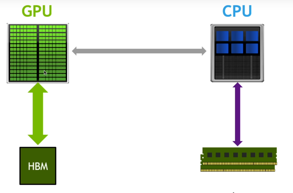
在 GPU 架构中,GPU 负责运算,显存负责存储,如果数据操作没有进行优化,则会导致数据在 GPU 和 HBM 之间被反复传输,极大地消耗了 I/O 资源,在使用 torch.compile() 优化后,会尽可能减少传输次数,提高 I/O 利用效率
# 在model被创建后执行
model = GPT(config=GPTConfig())
model.to(device)
model = torch.compile(model=model, backend='cudagraphs')使用后:dt: 69.50 ms, tok/ms: 1841.74(修改了 batch_size,所以和之前的数据无法对比)
Attention
不知道为啥,这里我使用默认的
inductor后端执行后一直报错,无法进行编译,好像是没有安装Triton,怎么也没有调试好,后来更换了后端为cudagraphs
step 3: Flash Attention
在 torch.compile() 中,对于某些函数是无法进行优化的,例如下面这个在 attention 中计算注意力分数的过程:
att = (q @ k.transpose(-2, -1)) * (1.0 / math.sqrt(k.size(-1)))
att = att.masked_fill(self.bias[:, :, :T, :T] == 0, float('-inf'))
att = F.softmax(att, dim=-1)
y = att @ v  # (B, nh, T, T) x (B, nh, T, hs) -> (B, nh, T, hs
所以采用了 Flash Attention 算法来替代这段代码(现在好像已经出到 v2 了):
y = F.scaled_dot_product_attention(q, k, v, is_causal=True)使用后提升:dt: 98.46 ms, tok/ms: 10400.07
step 4: Change Number
在模型训练过程中,我们期望一些 2 的幂次方,这样有利于模型的优化,在 GPT-2 中默认 vocab_size=50257 就是一个非常难优化的数字,因此我们需要改为 vocab_size=50304,训练速度为:dt: 106.32 ms, tok/ms: 9631.72
model = GPT(config=GPTConfig(vocab_size=50304))在训练过程中,会先将分好块的数据进行计算,如果没有剩余块就会直接输出结果,如果还有剩余块则会再来处理剩余部分,如果没能划分好则会大大减慢处理速度
训练参数设置
优化器参数
optim = AdamW(model.parameters(), lr=3e-4, betas=(0.9, 0.95), eps=1e-8)
梯度裁剪
norm = torch.nn.utils.clip_grad_norm_(model.parameters(), 1.0)
在叠加多层神经网络时,容易出现梯度爆炸的情况, 导致数值不稳定,因此考虑使用梯度裁剪的方式预防梯度爆炸,非常建议你打印出结果 norm(这是一个裁剪前的范数),如果 norm 在训练中不断升高,说明训练过程会很不稳定
如果梯度长度超过 ,那么拖影回长度 ,即:
李沐的书中有更详细的解释:8.5.5. 梯度裁剪
学习率调度器
在 GPT-2 中采用的是 cos_decay_with_warm_up
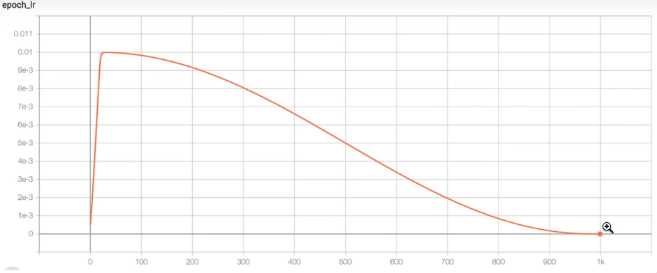
def get_lr(it):

    # 1) linear warmup for the first 10 steps
    if it < warmup_steps:
        return max_lr * (it+1) / warmup_steps
    # 2) min_lr for the rest of the steps
    if it > max_steps:
        return min_lr
    # 3) cosine decay for the training steps
    decay_ratio = (it - warmup_steps) / (max_steps - warmup_steps)
    assert 0 <= decay_ratio <= 1
    coeff = 0.5 * (1.0 + math.cos(math.pi * decay_ratio))
    return min_lr + coeff * (max_lr - min_lr)
权重衰减
对于一些 1 维参数,我们不需要权重衰减(例如:所有的 bias 参数,Layer Norm 中的参数等),因此需要对参数进行拆分
def configure_optimizers(self, weight_decay, learning_rate, device):
        param_dict = {pn:p for pn, p in self.named_parameters()}
        param_dict = {pn:p for pn, p in param_dict.items() if p.requires_grad}

        decay_params = [p for n, p in param_dict.items() if p.dim() >= 2]
        nodecay_params = [p for n, p in param_dict.items() if p.dim() < 2]

        optim_groups = [
            {'params': decay_params, 'weight_decay': weight_decay},
            {'params': nodecay_params, 'weight_decay': 0.0}
        ]

        num_decay_params = sum(p.numel() for p in decay_params)
        num_nodecay_params = sum(p.numel() for p in nodecay_params)
        print(f'num decay params: {len(decay_params)}, with {num_decay_params:,} parameters')
        print(f'num nodecay params: {len(nodecay_params)}, with {num_nodecay_params:,} parameters')

        fused_available = 'fused' in inspect.signature(torch.optim.AdamW).parameters
        use_fused = fused_available and 'cuda' in device
        print(f'using fused AdamW: {use_fused}')

        optim = torch.optim.AdamW(optim_groups, lr=learning_rate, betas=(0.9, 0.95), eps=1e-8, fused=use_fused)
        return opti
梯度累积
这里主要针对 GPU 算力不够的情况,可以使用 Gradient Accumulate 复现论文中的大 batch_size,但代价是更长的处理时间(并行变为串行)
total_batch_size = 524288 # 2**19, ~0.5M tokens
B = 1
T = 1024
assert total_batch_size % (B*T) == 0, "total_batch_size must be divisible by B*T"
grad_accum_steps = total_batch_size // (B*T)
print(f'total desired batch size: {total_batch_size}')
print(f'=> calculated gradient accumulation steps: {grad_accum_steps}'
代码部分比较简单,基本原理就是把之前的一个大 batch 拆分为多个小 batch,之后通过多次累积梯度后再更新一次参数
for step in range(max_steps):
    t0 = time.time()
    optim.zero_grad()
    for micro_step in range(grad_accum_steps):
        x, y = train_loader.next_batch()
        x, y = x.to(device), y.to(device)

        with torch.autocast(device_type=device, dtype=torch.bfloat16):
            logits, loss = model(x, y)
        loss = loss / grad_accum_steps # 这里需要特别注意
        loss.backward()
    norm = torch.nn.utils.clip_grad_norm_(model.parameters(), 1.0)
Attention
在累积的过程中,需要注意
loss的生成,如果是micro_step默认不会取平均,因此要加一个loss = loss / grad_accum_steps作为 normalization 方法
优化完后就是下面这样:
for step in range(max_steps):
    t0 = time.time()
    optim.zero_grad()
    loss_accum = 0.0
    for micro_step in range(grad_accum_steps):
        x, y = train_loader.next_batch()
        x, y = x.to(device), y.to(device)

        with torch.autocast(device_type=device, dtype=torch.bfloat16):
            logits, loss = model(x, y)
        loss = loss / grad_accum_steps
        loss_accum += loss.detach()
        loss.backward()
    norm = torch.nn.utils.clip_grad_norm_(model.parameters(), 1.0)
    # set learning rate
    lr = get_lr(step)
    for param_group in optim.param_groups:
        param_group['lr'] = lr
    optim.step()
    torch.cuda.synchronize()  # only needed with CUDA
    t1 = time.time()
    dt = (t1 - t0) * 1000  # ms
    tokens_per_sec = (train_loader.B * train_loader.T) / (t1-t0)
    print(
        f'step {step:4d}, loss: {loss_accum.item():.6f}, lr: {lr:.4e}, norm: {norm:.4f}, dt: {dt:.2f} ms, tok/ms: {tokens_per_sec:.2f}')
分布式训练
在视频当中使用的是 Distributed Data Parallel (DDP),核心思想简单来说就是数据并行,模型复制:
- 数据并行:
- 将输入数据分割成多个子集,每个 GPU 或节点处理一个子集。
- 每个 GPU 上都有一个完整的模型副本,独立计算前向传播和反向传播。
- 梯度同步:
- 在反向传播后,所有 GPU 上的梯度会通过通信(如 NCCL、Gloo)进行同步。
- 同步后的梯度用于更新模型参数,确保所有 GPU 上的模型保持一致。